
Perceptrons, Neural Networks and Dynamical Systems
By Sergi Andreu
// This post is last part of the “Deep Learning and Paradigms” post
Binary classification with Neural Networks
Neural Networks as homeomorphisms
Theorem 1 (Sufficient condition for invertible ResNets [1]):
Let \hat{\mathcal{F}} \, : \, \mathbb{R}^{d} \rightarrow \mathbb{R}^{d} with \hat{\mathcal{F}} (\cdot )= ( L^{1}_{\theta} \, \circ ... \circ \, L^{T}_{\theta} ) denote a ResNet with blocks defined by
L^{t} _{ \theta } = \mathbb{I} + h \cdot g_{\theta _t}
Then, the ResNet \hat{\mathcal{F}}_{\theta} is invertible if
h \cdot \text{Lip} (g_{\theta_t}) < 1 \text{ for all } t = 1, ..., T
We expect the lipschitz constant of g_\theta to be bounded, and so h\to 0 would make our ResNets invertible.
Neural Networks and Dynamical Systems
From what we have seen, now the relation between Neural Networks and Dynamical Systems is just a matter of notation!
– Consider the multilayer perceptron, given by
F(x) = f^L \circ f^{L-1} \circ ... \circ f^0 (x)
Simply renaming the index l by the index t-1, and L by T-1, we see that
F(x) = f^T \circ ... \circ f^t \circ ... \circ f^1 (x)If we define x_t = f^t \circ ... \circ f^0 (x), we see that what the neural network is doing is defining a dynamical system in which our initial values, denoted by x, evolve in a time defined by the index of the layers.
However, this general discrete maps are not easy to characterize. We can see that we are more lucky with ResNets*.
– In the case of Residual Neural Networks, the residual blocks are given by
f^t (x_{t-1}) = x_{t-1} + A^{t} x_{t-1} + b^t
where the supindex in A and b denote that A and b, in general, change in each layer.
Defining the function G(x, t) = (A^t (x) + b^t)/h, we can rewrite our equation as
x_{t+1} = x_{t} + h\cdot G(x_t, t)with the initial condition given by our input data (the ones given by the dataset).
Remember that the index t refers to the index of the layer, but can be now easily interpreted as a time.
In the limit h\to 0 it can be recasted as
\lim_{h \to 0} \frac{x_{t+1}-x_{t}}{h} = \dot{x}_t = G(x_t, t)and, since the discrete index t becomes continuous in this limit, it is useful to express it as
\dot{x}(t) = G(x(t), t)
This dynamic should be such that x(0) is the initial data, and x(T) is a distribution such that the points that were in M^0 and M^1 are now linearly separable.
Therefore the ResNet architecture can be seen as the discretization of an ODE, and so the input points x are expected to follow a smooth dynamics layer-to-layer, if the residual part is sufficiently small.
The question is: is the residual part sufficiently small? Is h indeed small? There are empirical evidence showing that, as the number of layers (T) incresases, the value h gets smaller and smaller.
But we do not need to worry too much, since we can easily define a general kind of ResNets in which the residual blocks are given by
f^t (x_{t-1}) = x_{t-1} + h (A^{t} x_{t-1} + b^t)in which h could be absorbed easily by A and b.
Deep Learning and Control
Recovering the fact that f^t are indeed f^t( \cdot ;\theta ^t), where $\theta^t$ are the parameters A^t and b^t, we can express our dynamical equations, in the case of resnets as
\dot{x}(t) = G(x(t), t; \theta (t))where x(0) is our initial data point, and we want to control our entire distribution of initial datapoints into a final suitable distribution, given by x(T). In the case of binary classification, that “suitable distribution” would for example consist in one in which the datapoints labelled as 0 move further away from the datapoints labelled as 1, yielding a final space that could be separated by an hyperplane.
Exploiting this idea, we have the Neural Ordinary Differential Equations [10].
Visualizing Deep Learning
In a binary classification problem using Deep Learning, we essentially apply the functions f\in \mathcal{H}, where \mathcal{H} has been previously defined, to our input points x, and then the space f(x) is divided by two by an hyperplane: one of the resulting subspaces would be classified as 0, and the other as 1.
Therefore, our problem consists on making an initial dataset linearly separable.
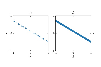
Consider a binary classification problem with noisless data, such that
\mathcal{D} = \{ ( x_i , y_i = \mathcal{F}(x_i) )\} _{i=1}^{S} x_i \in [-1,+1]^{n} , \; \; y_i \in \{0,1\} \quad \forall i \in \{1, ... , S\}We consider two distributions, the ring distribution and the spiral distribution.
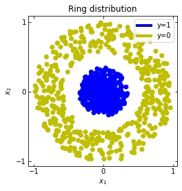
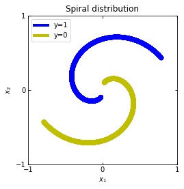
Plot of the ring and spiral distribution
And let’s put into practice what we have learned! For that, we use the library TensorFlow [14], in which we can easy implement the Multilayer Perceptrons and Residual Neural Networks that we have defined.
We are going to look at the evolution of x(t), with x(0) the initial datapoint of the dataset. Remember that we have two cases
– In a multilayer perceptron, x(t) = x_t = f^t \circ f^{t-1} \circ ... \circ f^1(x).
– In a ResNet, x(t) would be given by x(t+1) = x(t) + f(x(t)) that is, approximately, \dot{x}(t) = G(x(t), t).
Multilayer Perceptrons
In the case of multilayer perceptrons, we choose neurons per layer. This means that we are working with points in .
We train the networks, and after lots of iterations of the gradient descent method, this is what we obtain.

We see that in the final space (hidden layer 5) the blue and yellow points can be linearly separable.
However, the dynamics is far from smooth, and we see that in the final layers we seem to occupy a
dimensional space rather than a dimensional one. This is because multilayer perceptrons tend to “lose information”. This type of behaviour causes that if we had increased the number of layers this architectures would be super difficult to train (we would have to try lots of times, since each time we initialize the parameters at random).
Visualizing ResNets
With ResNets we are far luckier!
Consider two neurons per layer. That is, we would be working with in
.
We observe that altough the spiral distribution can be classified by this neurons (the transformed space, in hidden layer makes the distribution linearly separable) this does not happen with the ring distribution!
We should be able to respond why this happens with what we have learned: since the ResNets are homeomorphisms, we would not be able to untie the tie in the ring distribution!
However, we should be able to untie it if going to a third dimension. Let’s try that.
Now we consider neurons per layer, i.e.
.
Now both distributions can be classified. Indeed, every distribution in a plane could be in principle classified by a ResNet, since at most we would have ties of order , that can be untied in a dimension .
But could indeed all distributions be classified? Are the ResNets indeed such powerful approximators that we could recreate almost any dynamics out of them? Are we able to find the parameters
(that can be seen as controls) such that all distributions can be classified? What do we gain by increasing (having more and more layers)?
Those and far more other questions arise out of this approach. And those cannot be answered easily without further research.
Results, open questions and perspectives
Noisy vs noisless data
Considering the distribution in the figure (that can be seen as a more “natural” ring distribution), if we only cared about moving the blue points to the top, and the yellow points to the bottom, we would have an inecessary complex dynamics, since we expect some points to be mislabelled.
We should stick to “simple dynamics”, that are the ones we expect would generalise well. But how to define “simple dynamics”? In an optimal control approach, this has to do with adding regularization terms.
Moreover, Weinan E. et al [2] propose the approach of considering, instead of our points
as objects of study for the dynamics, the probabilty distribution, and so recasting the control as a mean field optimal control. With this approach, some we gain some insight into the problem of generalization.
This has to do with the idea that indeed what the Neural Networks take as inputs are probabilty distributions, and the dynamics should be focused on those. In here theories such as transportation theory try to give some insight into happens when consider the more general problem of Deep Learning: one in which we have noise.
Complexity and control of Neural Networks
We also do not know what happens when increasing the number of layers. Why increasing the number of layers is better?
In practice, having more layers (working in the so called overparametrization regime) seems to perform better in training. Our group indeed gave some insight in that direction [15] by connecting this problems with the turnpike phenomenon [16].
Regarding optimality, it is not easy to define, since we have multiple possible solutions to the same problem. That is, there are multiple dynamics that can make an initial distribution linearly separable.
It also seems that one should take into account some problem of stochastic control, since the parameters
are initialized at random, and different initializations give different results in practice. Moreover, the stochastic gradient descent, which is widely used, introduces some randomness to our problem. This indicates that Deep Learning is by no means a classical control problem.
Conclusions
Altough the problem of Deep Learning is not yet resolved, we have made a some very interesting equivalences:
- The problem of approximation in Deep Learning is now the problem of how is the space of possible dynamics? In the case of multilayer perceptrons, we can make use of discrete dynamical systems to solve that, or characterize their complexity; and in the case of ResNets, papers such at the one by Q. Li et. deals with that question [7].
- The problem of optimization is the problem of finding the best weights
- , that can be recasted as controls. That is, is a problem of optimal control, and we should be able to use our knowledge of optimal control (for example, the method of succesive approximations) in this direction.
- The generalization problem can be understood by consdering the control of the whole probability distribution, instead of the risk minimization problem [2].
All in all, there is still lot of work to do to understand Deep Learning.
However, the presented approaches have been giving very interesting results in the recent years, and everything indicates that they will continue to do so.
|| Go to the Math & Research main page


