Deep Learning and Paradigms
By Sergi Andreu
// This post is the 2nd. part of the “Opening the black box of Deep Learning” post
Deep Learning
Now that we have some intuition about the data, it’s time to focus on how to approximate the functions f that would fit that data.
When doing *supervised learning*, we need three basic ingredients:
– An hypothesis space, \mathcal{H}, consisting on a set of trial functions. All the functions in the hypothesis space can be determined by some parameters \theta. That is, all the functions f \in \mathcal{H} are given by f ( \cdot ; \theta ). We therefore want to find the best parameters \theta ^*.
– A loss function, that tells us how close we are from our desired function.
– An optimization algorithm, that allows us to update our parameters at each step.
Our algorithm consists on initializing the process by choosing a function $f( \cdot , \theta) \in \mathcal{H}$. In Deep Learning, this is done by randomly choosing some parameters \theta _0, and initializing the function as f( \cdot ; \theta_0).
In Deep Learning, the loss function is given by the empirical risk. That is, we choose a subset of the dataset, \{x_j , y_j\}_{j=1}^{s} and compute the loss as \frac{1}{s} \sum_{j=1}^{s} l_j ( \theta), where l_j could be simply given by l_j = \| f(x_j, \theta) - y_j \|_2^2.
The optimization algorithms used in Deep Learning are mainly based in Gradient Descent, such as
\theta_{k+1} = \theta_k - \epsilon \frac{1}{n} \nabla l_j ( \theta _k)
Where the subindex denotes the parameters at each iteration.
We expect our algorithm to converge; that is, we want that, as k \to \infty, we would have \theta_{k} close to \theta^*, where the notion of “closeness” is given by the chosen loss function.
Paradigms of Deep Learning
There are many questions about Deep Learning that are not yet solved. Three of that paradigms, that would be convenient to treat mathematically, are:
– Optimization: How to go from the initial function, F_0, to a better function \tilde{F}? This has to do with our optimization algorithm, but also depends on how do we choose the initialization, F_0.
– Approximation: Is the ideal solution F^* in our hypothesis space \mathcal{H}? Is \mathcal{H} at least dense in the space of feasible ideal solutions F^*? This is done by characterizing the function spaces \mathcal{H}.
– Generalization: How does our function \tilde{F} generalise to previously unseen data? This is done by studying the stochastic properties of the whole distribution, given by the generalised dataset.
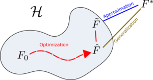
Diagram of the three main paradigms of Deep Learning. The function F_0 is the initial one, \tilde{F} is the final solution as updated by the optimization algorithm, \hat{F} is the closest function in \mathcal{H} to F^*, and F^* is the best ideal solution
The problem of approximation is somehow resolved by the so-called Universal Approximation Theorems (look, for example, at the results by Cybenko [11]). This results state that the functions generated by *Neural Networks* are dense in the space of continuous functions. However, in principle it is not clear what do we gain by increasing the number of layers (using *deeper Neural Networks*), that seem to give better results in practice.
Regarding optimization, altough algorithms based in Gradient Descent are widely used, it is not clear whether the solution gets stucked in local minima, if convergence is guaranteed, how to initialize the functions…When dealing with generalization, everything gets more complicated, because we have to derive some properties of the generalised dataset, from which we do not have access. It is probably the less understood of those three paradigms.
Indeed, those three paradigms are very connected. For example, if the problem of optimization is completely solved, we would know that our final solution given by the algorithm, \tilde{F}, would be the best possible solution in the hypothesis space, \hat{F}; and if approximation is solved, we would also end up getting the ideal solution F^*.
One of the main problems regarding those questions is that the hypothesis space \mathcal{H} is generated by a Neural Network, and so it is quite difficult to characterize mathematically. That is, we do not know much about the shape of \mathcal{H} (although the Universal Approximation Theorems give valuable insight here), nor how to “move” in the space \mathcal{H} by tuning \theta.
Let’s take a look at how the hypothesis spaces look like.
Hypothesis spaces
In classical settings, an hypothesis space is often proposed as
\mathcal{H} = \left\{ f (x\, ; \mathbf{\theta }) \; \bigg\vert f(x ; \theta ) = \sum_{i=1}^{m} a_i \psi _i (x) \right\}
where \theta = \{ a_i \}_{i=1}^{m} are the coefficients, \{ \psi _i\} are the proposed functions (for example, they would be monomials if we are doing polynomial regression).
The function \mathcal{F} correspondent to the dataset \mathcal{D} is then defined as
\mathcal{F}(\cdot ) \equiv f(\cdot \, ; \theta ^*) \in \mathcal{H} \quad \text{such that} \quad \theta ^* = \argmin \sum_{i=1}^{S} d(\phi (f(x_i \, ; \theta )) , y_i)
where d is a distance defined by a loss function, and \phi is a function that transforms f(x_i; \theta) such that we can compare it with y_i. For example, if we want to do binary classification, we would use \phi as a function that divides the space into two hiperplanes, and assigns $0$ to one of the parts of the divided space, and 1 to the other.
This means hat f(\cdot ; \theta^*) it is the function in the hypothesis space that minimizes the distance with the target function, which connects the datapoints x_i with their correspondent labels y_i.
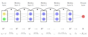
When using Deep Neural Networks, the hypothesis space \mathcal{H} is generated by the composition of simple functions f such that
\mathcal{H} = \left\{ f(x \, ; \theta ) \; \bigg\vert f(x ; \theta ) = \phi \circ f_{\theta_L}^L \circ f_{\theta_{L-1}}^{L-1} \circ ... \circ f_{\theta_1}^1 (x) \right\}
where \theta = \{ \theta_k \}_{k=1}^{L} are the training weights of the network and L the number of hidden layers.
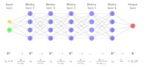
Multilayer perceptrons
In the case of the so-called multilayer perceptrons, the functions f^k_{\theta_k} are constructed as
f^k_{\theta_k} (\cdot) = \sigma (A^k (\cdot) + b^k)
being A^k a matrix, b^k a vector, \theta _k = \{A^k , b^k\} and \sigma \in C^{0,1}(\mathbb{R}) a fixed nondecreasing function, called the activation function.
Since we restrict to the case in which the number of neurons is constant through the layers, we have that A^k \in \mathbb{R}^{d \times d} and b^k \in \mathbb{R}^d.
Diagram of a multilayer perceptron, also called fully-connected neural network. However, this graph representation seems a bit difficult to treat, so we use an algebraic representation instead.
That is, sistematically, one has that \mathcal{H} = \{ F : F(x) = F_T \circ F_{T-1} \circ ... \circ F_0 (x) \}, the hypothesis space is generated by the discrete composition of functions.
It can be seen that the complexity of the hypothesis spaces in Deep Learning is generated by the composition of functions. Unfortunately, the tools regarding the understanding of the discrete composition of functions are quite limited.
Moreover, considering b^k=0, we have that F(x) = \sigma \circ A_T \circ \sigma \circ A_{T-1} \circ ... \circ \sigma A_0 \circ x. The gradient would then go as \nabla_\theta F \sim A_T \cdot A_{T-1} \cdot ... \cdot A_0 \sim k^L. For L large, the gradients would become very large or very small, and so training would not be feasible by gradient descent.
This is one of the reasons for introduction the Residual Neural Networks.
Residual Neural Networks
In the simple case of a Residual Neural Network (often referred to as ResNets) the functions f_{\theta_k}^{k} (\cdot) are constructed as
f_{\theta_k}^{k} (\cdot) = \mathbb{I} (\cdot) + \sigma (A^k (\cdot) + b^k)
where \mathbb{I} is the identity function. The parameters \sigma, A^k and b^k are equivalent to those of the multilayer perceptrons.
We will see that it is sometimes convenient to numerically add a parameter h to the residual block, such that
f_{\theta_k}^{k} (\cdot) = \mathbb{I} (\cdot) + h \, \sigma (A^k (\cdot) + b^k)
being h \in \mathbb{R} a scalar.
Diagram of a ResNet, in a graph manner. Again, an algebraic representation is preferred.
Visualizing Perceptrons
The Neural Networks then represent the compositions of functions f, which consist on an affine transformation plus a nonlinearity.
If we use the activation function \sigma ( \cdot ) = tanh (\cdot), then each function f (and so each layer of the Neural Network) is first rotating and translating the original space, and then “squeezing” it.
Example of the transformation of a regular grid by a perceptron
// This post continues on post: Perceptrons, Neural Networks and Dynamical Systems
References
[1] J. Behrmann, W. Grathwohl, R. T. Q. Chen, D. Duvenaud, J. Jacobsen.
Invertible Residual Networks (2018)
[2] Weinan E, Jiequn Han, Qianxiao Li.
A Mean-Field Optimal Control Formulation of Deep Learning. Vol. 6. Research in the Mathematical Sciences (2018)
[4] B. Hanin.
Which Neural Net Architectures Give Rise to Exploding and Vanishing Gradients? (2018)
[5] C. Olah.
Neural Networks, Manifolds and Topology [blog post]
[6] G. Naitzat, A. Zhitnikov, L-H. Lim.
Topology of Deep Neural Networks (2020)
[7] Q. Li, T. Lin, Z. Shen.
Deep Learning via Dynamical Systems: An Approximation Perspective (2019)
[8] B. Geshkovski.
The interplay of control and deep learning [blog post]
[9] C. Fefferman, S. Mitter, H. Narayanan.
Testing the manifold hypothesis [pdf]
[10] R. T. Q. Chen, Y. Rubanova, J. Bettencourt, D. Duvenaud.
Neural Ordinary Differential Equations (2018)
[11] G. Cybenko.
Approximation by Superpositions of a Sigmoidal Function [pdf]
[12] Weinan E, Chao Ma, S. Wojtowytsch, L. Wu.
Towards a Mathematical Understanding of Neural Network-Based Machine Learning_ what we know and what we don’t
[14]
Introduction to TensorFlow [tutorial]
[15] C. Esteve, B. Geshkovski, D. Pighin, E. Zuazua.
Large-time asymptotics in deep learning
[16]
Turnpike in a Nutshell [Collection of talks]
You might like!


