Collective dynamics modelling, Control and Simulation

Collective dynamics

Herds, packs, bird ﬂocks, and ﬁsh schools are common examples of the collective behaviors arising from the interactions of individuals. Each individual has its own decision policy, as in the stock market or game theory, which interacts with other participants.

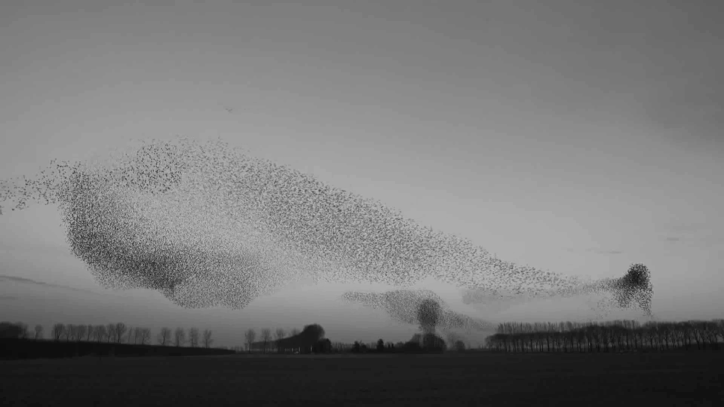
Figure 1. from National Geographic, 15 Nov 2016

Hence, in recent literature arising from statistical physics and mathematical biology, the modeling of the collective dynamics has focused on the interactions itself and assumes homogeneous individuals in general. Cucker-Smale model [1]:

$\begin{aligned} &{\dot {{\mathbf{x}}_i}}= {\mathbf{v}}_i, \quad t > 0, \quad i =1, \cdots, N, \\ &{\dot {{\mathbf{v}}_i}} = \frac{\kappa}{N} \sum_{j=1}^{N} \psi(\|{\mathbf{x}}_j - {\mathbf{x}}_i\|) ({\mathbf{v}}_j - {\mathbf{v}}_i), \\ &({\mathbf{x}}_i, {\mathbf{v}}_i)(0) = ({\mathbf{x}}_{i0}, {\mathbf{v}}_{i0}), \end{aligned}$

where $\kappa$ is the coupling strength, and the communication weight $\psi: {\mathbb R}_+ \to {\mathbb R}$ is the interaction function, for example, a positive constant. Note that we cannot distinguish individuals from the interactions since everyone has the same policy for its future motion from others’ data. This is a signiﬁcant diﬀerence from the concept of agent-based model in complex systems. Then, in such systems, what is the collective dynamics? It appears in the model as a long-time behavior, for example, the frequencies in the Kuramoto model converges to the same value if $\kappa$ is large enough.

Modeling problems

Then, what is a proper construction of interactions? Since the exact derivation of the equation is hidden in most applications of complex systems, we need to rely on heuristic methods, which can list as follows:

• Extend and simplify the observation from few individuals; for example, from voltage exchanges of cells (Peskin model [2]).

• Focus on the basic interactions; the alignment of velocities (Cucker-Smale model [1])

• Use Optimization; build an objective function ﬁrst, and then consider its gradient ﬂow. (Kuramoto model [3])

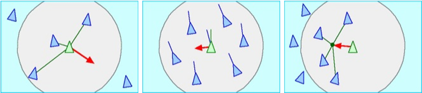
Figure 2. Interaction rules from Craig Reynolds [4]

Control problems

The objective of the control in collective dynamics is rather natural; we want to change the collective dynamics as we want. Still, one of the main questions remains in the importance of a large crowds of interacting agents since we are dealing with huge number of individuals, the controls are commonly required to be constructed by a low-dimensional strategy [5]. One may control many individuals with the same control function, or few individuals with dedicatedly determined control functions [6].

For example, how can we control the consensus network from the opinion of one individual? [7] How can we ﬁnd the locomotion of a few shepherd dogs which manages a lot of sheep? In this herding problem, we don’t want to control the sheep one by one; we use the dogs to steer them as a herd [8].

Simulations

If we cannot establish simple feedback strategies, a natural and classical strategy is to ﬁnd the optimal control, which is the control function minimizing an objective function, such as the deviation of sheep’s position or the distance of them to the target position. In numerical simulations, following the calculations of variations, the minimizer can be found by tracking the gradient of the objective function.

For a large number of individuals, the simulations on optimal controls needs a huge computation power and becomes unfeasible easily. How much computing power we need to simulate, hundreds, thousand, or millions of particles? Hence, the model reduction of collective behavior models are required, for example, the mean-ﬁeld limit [9].

Remarks

Control in complex systems highly relies on the dynamical perspectives and speciﬁc properties of given models. Compared to the developed theory in PDE controls, it lacks estimations on the cost of control, controllability arguments, and the sensitivity analysis with diﬀerent control functions.

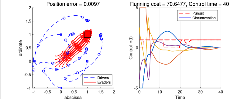
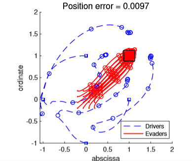
Figure 3. The simulation on four drivers (shepherd dogs) guiding sixteen evaders (sheep) from (0,0) to (1,1) presented in [8]

References

[1] F. Cucker and S. Smale, Emergent behavior in ﬂocks, IEEE Trans. Automat. Control 52 (2007) 852-862

[2] C. S. Peskin, Mathematical aspects of heart physiology, Courant Institute of mathematical sciences, (1975), pp. 268-278

[3] Y. Kuramoto, International Symposium on Mathematical Problems in Mathematical Physics, Lecture Notes in Theoretical Physics 30 (1975) 420

[4] C. W. Reynolds, Flocks, herds and schools: A distributed behavioral model. In Proceedings of the 14th annual conference on Computer graphics and interactive techniques (1987) 25–34

[5] M. Bongini, M. Fornasier, F. Rossi, F. Solombrino, Mean-Field Pontryagin Maximum Principle, Journal of Optimization Theory and Applications 1 (2017) 1–38

[6] M. Caponigro, M. Fornasier, B. Piccoli, E. Tr´elat, Sparse stabilization and optimal control of the CuckerSmale model, Mathematical Control and Related Fields 3(4) (2013) 447–466

[7] U. Biccari, D. Ko, E. Zuazua, Dynamics and control for multi-agent networked systems: a ﬁnite diﬀerence approach. Mathematical Models and Methods in Applied mathematics 29 4, (2019), 755-790

[8] D. Ko, E. Zuazua, Asymptotic behavior and control of a “guidance by repulsion” model. Mathematical Models and Methods in Applied Sciences, Online Ready. doi: 10.1142/S0218202520400047, 2020

[9] S.-Y. Ha, J.-G. Liu, A simple proof of Cucker-Smale ﬂocking dynamics and mean ﬁeld limit. Communications in Mathematical Sciences 7, (2009) 297–325